A probabilistic graphical model (PGM) is a graph that represents a joint distribution $p(\mathbf{x})$. The graph shows how the joint distribution factorizes and, equivalently, also shows the (conditional) independence relations between the variables. There are two main flavours of PGMs.

Directed PGMs (Bayesian networks)

A directed PGM uses a directed acyclic graph (DAG) to represent distributions. Each node is a variable. The joint distribution is the product of the conditional distribution of each node, given its parents:

The d-separation rules give the conditional and unconditional independence relations in the graph. The Markov blanket of a node contains its parents, its children and, because of explaining away, its co-parents.

Undirected PGMs (Markov random fields / Markov networks)

An undirected PGM uses an undirected graph. In this case, the joint distribution is written as the product of potential functions on the (maximal) cliques $C$ of the graph:

$Z$ is the partition function. Simple graph separation shows the independence relations. Thus, the Markov blanket of a node contains only its neighbours. If all potentials are strictly positive, each potential is an exponential of a negative energy function $E$:

The joint distribution is then a Gibbs-Boltzmann distribution. This is the form of energy-based models (EBMs).

Representational power

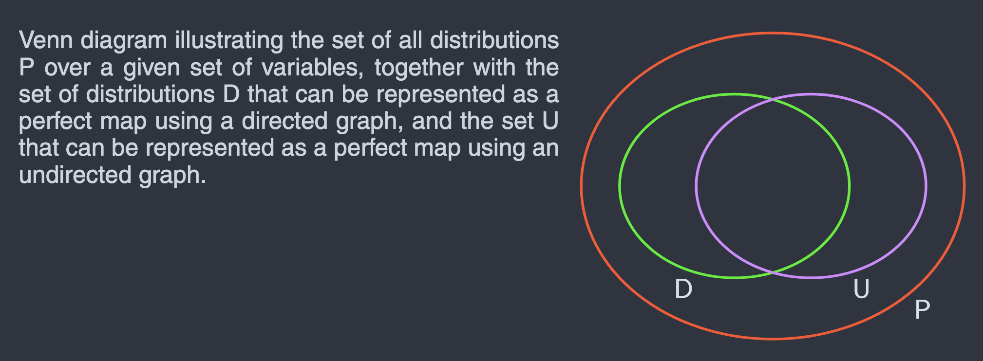
A PGM can show all the conditional independence relations of a distribution and no other relations. In this case, the PGM is said to be a perfect map of the distribution. Some distributions have a perfect map only as a directed graph and some have a perfect map only as an undirected graph. Some distributions have no perfect map of either type.

Also, a directed PGM and an undirected PGM can both represent the same distribution. Even then, the set of conditional independence relations that can be read out from each representation may be different. So these are incomplete representations of underlying distributions. Going even further, it's important to remember that distributions themselves are models of underlying phenomena, not the phenomena themselves.

Factor graphs

A factor graph shows the factorization more explicitly. It is a bipartite graph with one node for each variable and one node for each factor. Each factor node connects to the variables that the factor uses:

You can change each of the two flavours of PGM above into a factor graph. In a directed PGM, the factors are the conditional distributions $p(x_i\mid {\text{pa}}_i)$. In an undirected PGM, the factors are the clique potentials ${\psi }_C$.

A factor graph gives more detail than the above two flavours. For example, two or more factors can use the same set of variables. A factor graph can also remove some ambiguities. For example, a fully connected triangle in an undirected graph can be one three-way potential or three pairwise potentials. The undirected graph does not show the difference, but the factor graph can.

The main advantage of a factor graph is for inference. If the factor graph is a tree, the sum-product algorithm (belief propagation) calculates the exact marginals. The algorithm sends local messages between variable nodes and factor nodes. The marginal of a node is the product of the messages that come into that node. If you replace each sum with a maximum, you get the max-sum algorithm. This algorithm finds the most probable configuration (the Viterbi algorithm is a special case). On a graph with loops, you can use the same message passing (loopy belief propagation). The result is only approximate, but it is often good in practice.